Pytorch Tutorial

2022-06-14

To understand pytorch training codes better, I start to follow a full totorial and summarize my progress here.

Basic Concepts

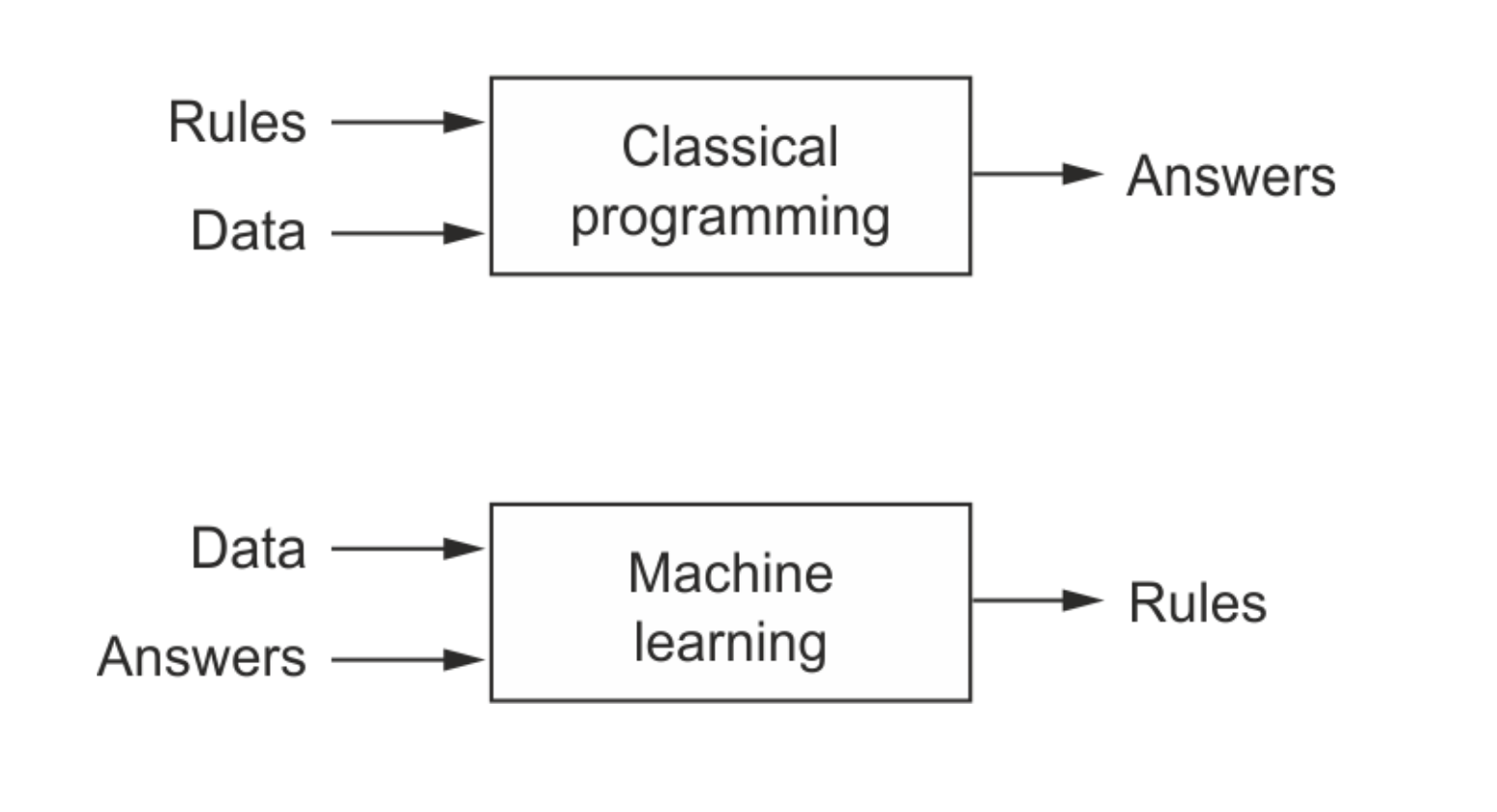
Unlike classical programming where we input data and algorithm (rules) to get the output, we give data and output to the ML training algorithm so that it can figure out the correct output for unknown data.

Tensor

all data elements of a tensor are converted to have the same type (e.g., float)
the shape of a tensor must be regular 3-dimension (difference from a simple list-of-list)

PyTorch

a library for tensor processing
the underlying implementation is in CUDA language (c language, which is fast), but it provides a layer of python wrappers (which is slow, but easy to use) of CUDA API calls
why it’s great? we can automatically compute the gradient (i.e., autograd using .backward()) of the output w.r.t. tensors
specify require_grad = True of a tensor to reduce unnecessary gradient calculation cost

Example:

# Create tensors.
x = torch.tensor(3.)
w = torch.tensor(4., requires_grad=True)
b = torch.tensor(5., requires_grad=True)
# Arithmetic Operation
y = w * x + b
# Compute gradients using autograd
y.backward()
# Display gradients
print('dy/dx:', x.grad)
print('dy/dw:', w.grad)
print('dy/db:', b.grad)

Output:

dy/dx: None
dy/dw: tensor(3.)
dy/db: tensor(1.)

PyTorch interoperates well with numpy, so we can use numpy to easily handle our data and also take benefit of PyTorch (Autograd, tensor operations on GPU).

Linear Regression (y = xW^T + b)

Linear regression is to a relationship between input variables (e.g., study time) and target variables (score). Each target variable is estimated to be a weighted sum of the input variables, offset by some constant (i.e., bias).

Here, learning means to figure out the weights using the training data. How? Gradient Descent: Just adjust slightly many times towards better accuracy.

To represent this problem mathematically, we form a matrix of the weights and vector of biases (# of target variables == # of rows).

Loss Function

to evaluate the model accuracy during training
typically use MSE (Mean Squared Error), why square? to remove negative values

Overall Process

Setup Model
Generate Predictions
Calculate Loss
Compute Gradients w.r.t. Weights and Biases
Adjust Weights and Biases
Reset Gradients to Zero (why? gradients are accumulated throughout training)

# Weights and biases
w = torch.randn(2, 3, requires_grad=True)
b = torch.randn(2, requires_grad=True)

# Setup model
def model(x):
    return x @ w.t() + b

# MSE loss
def mse(t1, t2):
    diff = t1 - t2
    return torch.sum(diff * diff) / diff.numel()

# Train for 100 epochs
for i in range(100):
    preds = model(inputs)
    loss = mse(preds, targets)
    loss.backward()
    with torch.no_grad(): # stop tracking operations while adjusting
        w -= w.grad * 1e-5
        b -= b.grad * 1e-5
        w.grad.zero_()
        b.grad.zero_()

** Note on torch.no_grad(): By default, PyTorch tracks all operations (during FP) on tensors with required_grad=True, which is called gradient context tracking by autograd engine. This tracking task has some processing and memory cost, so we deactivate it using torch.no_grad() when it’s not needed.

Linear Regression using PyTorch Built-in

the above training process is common, so several built-ins are provided

packages

from torch.utils.data import TensorDataset: allow us to handle certain rows (why? to handle data into batches, see below) of data as a tuple of (input, output)

from torch.utils.data import TensorDataset
# Define dataset
train_ds = TensorDataset(inputs, targets)
train_ds[0:3]

from torch.utils.data import DataLoader: split data into batches while shffuling

from torch.utils.data import DataLoader
# Define data loader
batch_size = 11
train_dl = DataLoader(train_ds, batch_size, shuffle=True) # why shffle? data might be sorted by default, but we want to train overall data

import torch.nn as nn: contains utility classes for building neural networks

import torch.nn as nn
# Define model
model = nn.Linear(3, 2) # 3 weights, 2 biases (3 inputs, 2 outputs)
print(model.weight)
print(model.bias)
# model.parameters() returns a list of tensors weight and bias

"""
Output:
Parameter containing:
tensor([[ 0.1312, -0.4246, -0.2341],
        [ 0.4099,  0.4766,  0.1676]], requires_grad=True)
Parameter containing:
tensor([ 0.1603, -0.0098], requires_grad=True)
"""

# Here, model is an object (not a function), but we can do FP in the same way
preds = model(inputs)

import torch.nn.functional as F: built-in loss function (e.g., mse_loss)

...
# Import nn.functional
import torch.nn.functional as F
# Define loss function
loss_fn = F.mse_loss
loss = loss_fn(model(inputs), targets)

torch.optim.SGD: optimize parameters using gradients instead of manually updating them (meaning of stochastic: batches are selected with random shuffling instead of the entire data)

# Define optimizer
opt = torch.optim.SGD(model.parameters(), lr=1e-5)
"""
tell the optimizer: "matrices model.parameters() need to be updated 
"""

Using all these built-ins, training model can be implemented again as follows:

...
# Utility function to train the model
def fit(num_epochs, model, loss_fn, opt, train_dl):
    
    # Repeat for given number of epochs
    for epoch in range(num_epochs):
        
        # Train with batches of data
        for xb,yb in train_dl: 
            # train_dl is a list of tuples of tensors (input, output), while each tensor has a batch of tensors
            
            # 1. Generate predictions
            pred = model(xb)
            
            # 2. Calculate loss
            loss = loss_fn(pred, yb)
            
            # 3. Compute gradients
            loss.backward()
            
            # 4. Update parameters using gradients
            opt.step()
            
            # 5. Reset the gradients to zero
            opt.zero_grad()
        
        # Print the progress
        if (epoch+1) % 10 == 0:
            print('Epoch [{}/{}], Loss: {:.4f}'.format(epoch+1, num_epochs, loss.item())) # loss is tensor of a single value, so loss.item retrieves the value

fit(100, model, loss_fn, opt, train_dl) # train for 100 epochs

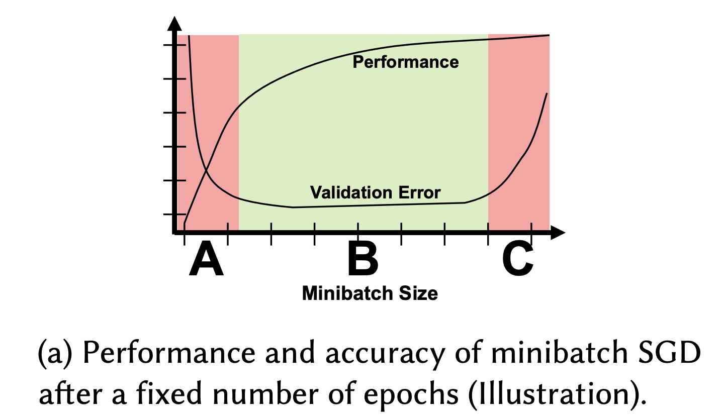
Note: why stochastic (batches with random shuffling) instead of the enrtire dataset?

memory: no need to fit the entire data at once
accuracy: gives more chances for convergence
total amount of computation should be the same eventually
performance will be lower though (due to less parallelization).

[source]

Logistic Regression for Image Classification

The problem setup is different from the linear regression as follows:

Input: a number of variables -> a single image
Output: a number of variables -> a single label
Example: a single MNIST data consist of one image and it’s label

However, PyTorch is a library to handle tensors, so we need to convert the images to tensors. It can be doen using torchvision.transform:

import torchvision # a package of utilities for working with image data
import torchvision.transforms as transforms
# MNIST dataset, 1 data = (image, label)
dataset = MNIST(root='data/', 
                train=True,
                transform=transforms.ToTensor())
img_tensor, label = dataset[0]

print(len(dataset), img_tensor.shape, label) 
# 60000, torch.Size([1, 28, 28]), 5

Then, we split the training dataset into training set and validation set, so that we can use different datasets for validation and training (note: MNIST has a separate dataset for test with 10000 images). What is the difference between validation and test? Validation is to evaluate the model during training and adjust hyperparameters (learning rate, etc.). Test is to measure the final accuracy and compare to other models.

from torch.utils.data import random_split

train_ds, val_ds = random_split(dataset, [50000, 10000])
len(train_ds), len(val_ds) # 50000, 10000

Then, we batch the data:

from torch.utils.data import DataLoader

batch_size = 128

train_loader = DataLoader(train_ds, batch_size, shuffle=True) # invoke shuffle for each epoch to randomize (i.e., generalize), which helps faster convergence   
val_loader = DataLoader(val_ds, batch_size) # no need to be shuffled (it's not for training)

We have prepared the dataset for training. Then, how can we set the model? Interestingly, the training model is conceptually the same as linear regression (y = xW^T + b). Each pixel (of 28*28) is weighted individually, to predict the probability of the image to be each label.

import torch.nn as nn

input_size = 28*28
num_classes = 10 # number of outputs (labels)

# Logistic regression model
model = nn.Linear(input_size, num_classes)
print(model.weight.shape) # torch.Size([10, 784])
print(model.bias.shape) # torch.Size([10])

However, one issue is that the input (image) and weight shape mismatch (1,28,28 vs 784). So, we reshape the input before we do FP. We can add this additional functionality by extending the default nn.Module class from PyTorch:

class MnistModel(nn.Module):
    def __init__(self):
        super().__init__()
        self.linear = nn.Linear(input_size, num_classes)
        
    def forward(self, xb):
        xb = xb.reshape(-1, 784)
        # by giving -1 for the first dimension, PyTorch automatically calculate it depending on the input, so we can use it with any batch size of xb 
        out = self.linear(xb)
        return out
    
model = MnistModel()

Now, we can use the model for FP:

for images, labels in train_loader:
    print(images.shape)
    outputs = model(images) # the base class nn.Module calls the forward() method by default
    break

print('outputs.shape : ', outputs.shape) 
# outputs.shape :  torch.Size([128, 10])
print('Sample outputs :\n', outputs[:2].data)
# Sample outputs :
# tensor([[ 0.0245,  0.0691, -0.1861,  0.1229, -0.1947, -0.1299,  0.1847, -0.2836, 0.2063, -0.1164], [-0.2538,  0.0495, -0.0900,  0.0783,  0.0670, -0.2608, -0.1726, -0.0452, 0.1272,  0.0451]])

Softmax: convert to probability

Then, we want to convert the output into probability of each label. For this, we use Softmax function provided by import torch.nn.functional as F:

# Apply softmax for each output row
probs = F.softmax(outputs, dim=1)

# Look at sample probabilities
print("Sample probabilities:\n", probs[:2].data)
# Sample probabilities:
# tensor([[0.1042, 0.1090, 0.0844, 0.1150, 0.0837, 0.0893, 0.1223, 0.0766, 0.1250, 0.0905], [0.0805, 0.1090, 0.0948, 0.1122, 0.1109, 0.0799, 0.0873, 0.0991, 0.1178, 0.1085]])
# Add up the probabilities of an output row
print("Sum: ", torch.sum(probs[0]).item())
# Sum:  0.9999999403953552

Now, we can calculate the accuracy of our model as follows:

def accuracy(outputs, labels):
    _, preds = torch.max(outputs, dim=1)
    # torch.max(dim=1) returns each row's largest element and the corresponding index.
    return torch.tensor(torch.sum(preds == labels).item() / len(preds))

Although this accuracy is intuitive to human, we cannot use it for loss function in gradient descent algorithm, because:

torch.max() and == are both non-continuous and non-differentiable operations
by taking only the final label with the maximum probability, it does NOT have enough insight about how to update the weights of each label (i.e., each column in W)

So, for the loss function in classification problems, we commonly use cross entropy instead. This cross entropy is also provided by torch.nn.functional, and it internally includes the softmax operation as well (we need to pass the raw output). For a batch of data, the cross entropy averages out over all data samples.

loss_fn = F.cross_entropy
# Loss for current batch of data
loss = loss_fn(outputs, labels)
# Interpretation: our model predicted the correct label with probability e^(-loss) in avg

Using the above logics, the overall training process is implemented as follows:

def evaluate(model, val_loader):
    outputs = [model.validation_step(batch) for batch in val_loader]
    return model.validation_epoch_end(outputs)

class MnistModel(nn.Module):
    def __init__(self):
        super().__init__()
        self.linear = nn.Linear(input_size, num_classes)
        
    def forward(self, xb):
        xb = xb.reshape(-1, 784)
        out = self.linear(xb)
        return out
    
    def training_step(self, batch):
        images, labels = batch 
        out = self(images)                  # Generate predictions
        loss = F.cross_entropy(out, labels) # Calculate loss
        return loss
    
    def validation_step(self, batch):
        images, labels = batch 
        out = self(images)                    # Generate predictions
        loss = F.cross_entropy(out, labels)   # Calculate loss
        acc = accuracy(out, labels)           # Calculate accuracy
        return {'val_loss': loss, 'val_acc': acc}
        
    def validation_epoch_end(self, outputs):
        batch_losses = [x['val_loss'] for x in outputs]
        epoch_loss = torch.stack(batch_losses).mean()   # Combine losses
        batch_accs = [x['val_acc'] for x in outputs]
        epoch_acc = torch.stack(batch_accs).mean()      # Combine accuracies
        return {'val_loss': epoch_loss.item(), 'val_acc': epoch_acc.item()}
    
    def epoch_end(self, epoch, result):
        print("Epoch [{}], val_loss: {:.4f}, val_acc: {:.4f}".format(epoch, result['val_loss'], result['val_acc']))
    
model = MnistModel()


def fit(epochs, lr, model, train_loader, val_loader, opt_func=torch.optim.SGD):
    optimizer = opt_func(model.parameters(), lr)
    history = [] # for recording epoch-wise results
    
    for epoch in range(epochs):
        
        # Training Phase 
        for batch in train_loader:
            loss = model.training_step(batch)
            loss.backward()
            optimizer.step()
            optimizer.zero_grad()
        
        # Validation phase
        result = evaluate(model, val_loader)
        model.epoch_end(epoch, result)
        history.append(result)

    return history

Limitations and Improvement

The above training algorithm works pretty well, but the accuracy improvement is saturated after about 80%. There are two potential reasons:

the learning rate is too high, so the model is “bouncing” around the optimal state
the linear model is not “powerful” enough

As one way to make the model more powerful, we can add one more layer along with a hidden layer (ReLU) to add non-linearity:

class MnistModel(nn.Module):
    """Feedfoward neural network with 1 hidden layer"""
    def __init__(self, in_size, hidden_size, out_size):
        super().__init__()
        # hidden layer
        self.linear1 = nn.Linear(in_size, hidden_size)
        # output layer
        self.linear2 = nn.Linear(hidden_size, out_size)
        
    def forward(self, xb):
        # Flatten the image tensors
        xb = xb.view(xb.size(0), -1)
        # Get intermediate outputs using hidden layer
        out = self.linear1(xb)
        # Apply activation function
        out = F.relu(out)
        # Get predictions using output layer
        out = self.linear2(out)
        return out
    
    def training_step(self, batch):
        images, labels = batch 
        out = self(images)                  # Generate predictions
        loss = F.cross_entropy(out, labels) # Calculate loss
        return loss
    
    def validation_step(self, batch):
        images, labels = batch 
        out = self(images)                    # Generate predictions
        loss = F.cross_entropy(out, labels)   # Calculate loss
        acc = accuracy(out, labels)           # Calculate accuracy
        return {'val_loss': loss, 'val_acc': acc}
        
    def validation_epoch_end(self, outputs):
        batch_losses = [x['val_loss'] for x in outputs]
        epoch_loss = torch.stack(batch_losses).mean()   # Combine losses
        batch_accs = [x['val_acc'] for x in outputs]
        epoch_acc = torch.stack(batch_accs).mean()      # Combine accuracies
        return {'val_loss': epoch_loss.item(), 'val_acc': epoch_acc.item()}
    
    def epoch_end(self, epoch, result):
        print("Epoch [{}], val_loss: {:.4f}, val_acc: {:.4f}".format(epoch, result['val_loss'], result['val_acc']))

Using a GPU

As the dataset and model are getting bigger, we use GPUs to train our model in a reasonable amount of time. First, let’s see how to move our data to GPU. We define a DeviceDataLoader which wraps the existing DataLoader and move the batches one by one to GPU.

def get_default_device():
    """Pick GPU if available, else CPU"""
    if torch.cuda.is_available():
        return torch.device('cuda')
    else:
        return torch.device('cpu')
def to_device(data, device):
    """Move tensor(s) to chosen device"""
    if isinstance(data, (list,tuple)):
        return [to_device(x, device) for x in data]
    return data.to(device, non_blocking=True)
class DeviceDataLoader():
    """Wrap a dataloader to move data to a device"""
    def __init__(self, dl, device):
        self.dl = dl
        self.device = device
        
    def __iter__(self):
        """Yield a batch of data after moving it to device"""
        for b in self.dl: 
            yield to_device(b, self.device)
            # Keyword 'yield'? It generates a value to be returned when the object is accessed. Here, one batch of data will be moved to GPU and returned every time this dala loader is accessed in for loop.

    def __len__(self):
        """Number of batches"""
        return len(self.dl)

device = get_default_device()
train_loader = DeviceDataLoader(train_loader, device)

Note that we are moving only the data batch to be trained at the time to GPU using yield keyworkd. It’s to reduce waste of GPU memories. Also, removing the trained data from GPU is automatically done by garbage collection.

Then, we move the model to the GPU:

1
2
3

# Model (on GPU)
model = MnistModel(input_size, hidden_size=hidden_size, out_size=num_classes)
to_device(model, device)

Convolutional Neural Network

To solve more complex problems using ML, we need to use more powerful models. CNN (nn.Conv2d) is one example of that.

Kernel and Convolution

Kernel: a matrix of weights
Convolution: an operation of sliding the kernel over the 2D input data, performing an elementwise multiplication, and then summing up the results into a single output pixel

For multi-channel images, a different kernel is applied to each channels, and the outputs are added together pixel-wise.

Advantages

Fewer parameters compared to FC layer where we have weight for every input element
Sparsity of connections since each output element depends on only a small part of input elements, which makes FP and BP more efficient
Parameter sharing by using the kernel trained in one part of input to detect a similar pattern in another part as well

Pooling

From each convolutional layer, we can use pooling layers to progressively decrease height & width of the output tensors

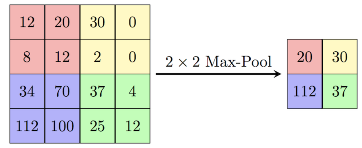
[source]

Note that there are several operations possible for pooling (e.g., max, avg).

Model

Using the convolution and pooling operations, we can form a CNN model as follows:

class Cifar10CnnModel(ImageClassificationBase):
    def __init__(self):
        super().__init__()
        self.network = nn.Sequential(
            nn.Conv2d(3, 32, kernel_size=3, padding=1),
            nn.ReLU(),
            nn.Conv2d(32, 64, kernel_size=3, stride=1, padding=1),
            nn.ReLU(),
            nn.MaxPool2d(2, 2), # output: 64 x 16 x 16

            nn.Conv2d(64, 128, kernel_size=3, stride=1, padding=1),
            nn.ReLU(),
            nn.Conv2d(128, 128, kernel_size=3, stride=1, padding=1),
            nn.ReLU(),
            nn.MaxPool2d(2, 2), # output: 128 x 8 x 8

            nn.Conv2d(128, 256, kernel_size=3, stride=1, padding=1),
            nn.ReLU(),
            nn.Conv2d(256, 256, kernel_size=3, stride=1, padding=1),
            nn.ReLU(),
            nn.MaxPool2d(2, 2), # output: 256 x 4 x 4

            nn.Flatten(), 
            nn.Linear(256*4*4, 1024),
            nn.ReLU(),
            nn.Linear(1024, 512),
            nn.ReLU(),
            nn.Linear(512, 10))
        
    def forward(self, xb):
        return self.network(xb)

Techniques for higher accuracy or better performance

Data Normalization

across each channel, subtract the mean, then divide by the standard deviation
prevent one channel with a higher or wider range of values affecting the final loss and gradients disproportionately
note that the same normalization (using the same stats) must be applied to validation and test dataset as well (since the model is trained on the normalized dataset)

Data Transformation

apply randomly chosen transformations, such as paddding & random crop, flipping, etc., while loading the data
generalize the model better
note that this transformation need to be applied to the training dataset only (since its to give more information to the training process)

# Data transforms (normalization & data augmentation)
import torchvision.transforms as tt
stats = ((0.4914, 0.4822, 0.4465), (0.2023, 0.1994, 0.2010))
train_tfms = tt.Compose([tt.RandomCrop(32, padding=4, padding_mode='reflect'), 
                         tt.RandomHorizontalFlip(), 
                         # tt.RandomRotate
                         # tt.RandomResizedCrop(256, scale=(0.5,0.9), ratio=(1, 1)), 
                         # tt.ColorJitter(brightness=0.1, contrast=0.1, saturation=0.1, hue=0.1),
                         tt.ToTensor(), 
                         tt.Normalize(*stats,inplace=True)])
valid_tfms = tt.Compose([tt.ToTensor(), tt.Normalize(*stats)])

DataLoader Parameters

num_workers to leverage multiple CPU cores in parallel
pin_memory to avid repeated memory allocation and deallocation by using the same portion of RAM for loading each batch (its possible when all the batches have the same size)

`1`	`train_dl = DataLoader(train_ds, batch_size, shuffle=True, num_workers=3, pin_memory=True)`

Reference

https://www.youtube.com/watch?v=GIsg-ZUy0MY

Previous AWS SageMaker

Next Operating Systems